Mesh adaptation

In this section, some examples of mesh adaptation are presented. In all of them, the following mesh (hole.mesh) is used.

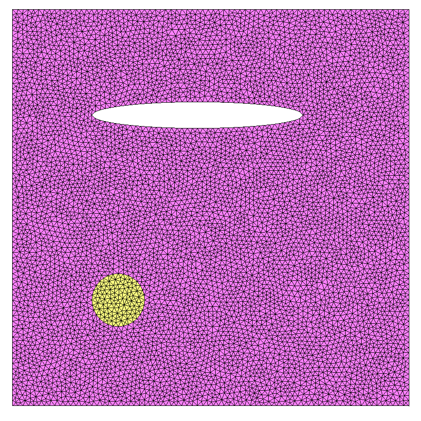
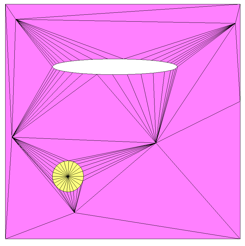
Initial mesh: a square with a hole and two different domains (different references)

Default parameters

To run mmg2d with default parameters, run the following command:

mmg2d_O3 hole.mesh

The output mesh, stored in a file called hole.o.mesh, is displayed below:

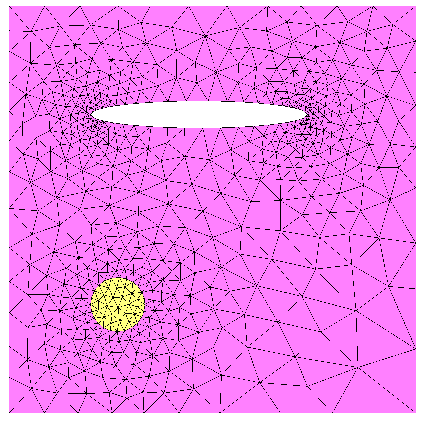
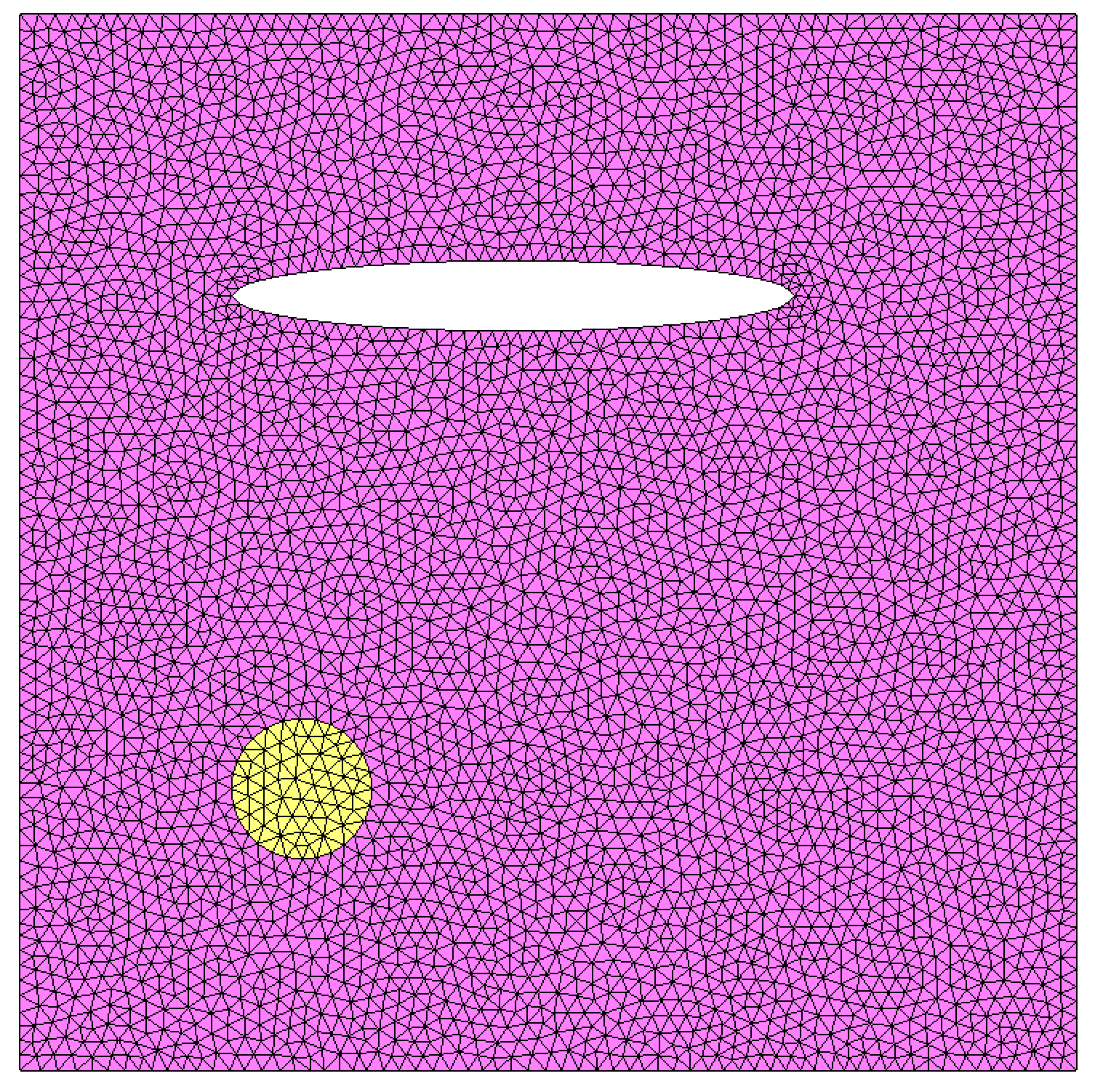
Output mesh with default parameters

mmg attempt to unrefine the mesh while:

• preserving the maximal distance between the ideal geometry and its discretization (set with -hausd option, equal to 0.01 by default).

• applying the prescribed gradation (set with -hgrad option, 1.3 by default) that enforces the maximal length ratio between two adjacent edges.

• preserving the subdomains.

Boundary approximation control

The boundary approximation is controlled by the Hausdorff parameter. The -hausd option allows to adapt the Hausdorff value. The mesh bounding box of this example is [-5 ; 10]x[-5 ; 10]. To set a maximal Hausdorff distance of 0.1, run the following command:

mmg2d_O3 -hausd 0.1 hole.mesh

This produces the following output:

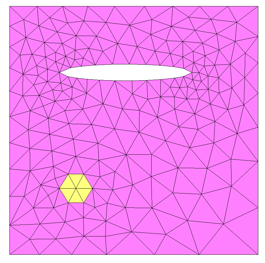
Output mesh for a Hausdorff parameter of 0.1.

In this example, the hole boundary and the interface between the two domains are degraded because the Hausdorff distance that has been set is large compared to the object sizes.

In general, note that:

• decreasing the Hausdorff parameter leads to refine the mesh in areas with high curvature.

• the ideal Hausdorff parameter depends of mesh size and the default value will rarely fit.

• knowing the mesh bounding box is very useful to fit the Hausdorff parameter. Visualizing a mesh with Medit is a good way to get the size of the bounding box.

• the default value of the Hausdorrf parameter is equal to 0.01 and is suitable for a circle of radius 1.

Gradation

The -hgrad parameter control the mesh gradation, i.e. the ratio between the lengths of two adjacent edges. By default, this parameter is set to 1.3.

It is possible to:

• customize the ratio value by passing it to the -hgrad option.

• disable the gradation by setting -hgrad -1.

The two following meshes are obtained by running the following commands:

mmg2d_O3 -hgrad 2.3 hole.mesh
mmg2d_O3 -hgrad -1  hole.mesh

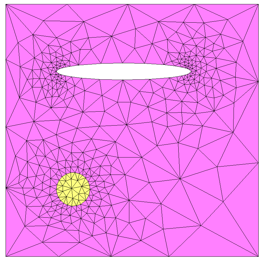
Output mesh with gradation set to 2.3

Output mesh without gradation

Note that disabling the gradation can lead to bad quality meshes.

Constant mesh size

A constant edge size may be prescribed using the -hsiz option:

mmg2d_O3 hole.mesh -hsiz 0.25

With this option, mmg produces a mesh that respects the intersection between the size map prescribed by the Hausdorff parameter and the constant size map provided with the option -hsiz, which amounts to keeping the smallest size.

This intersected size map still respects the gradation parameter.

Output mesh with constant mesh size of 0.25 (-hsiz 0.25)

Adaptation to an input size map

To enforce a desired mesh size that is variable over the initial mesh, it is possible to supply mmg with a size map. A size map is a scalar or tensorial function defined over mesh vertices. At each vertex, its value represent the target size of surrounding elements in the mesh.

Size maps may be provided in the following way:

• as a .sol file if the input mesh is in Medit file format .mesh. Mmg automatically detects the .sol file that has the same name as the input mesh. In this example, the file would be named hole.sol. Otherwise, it is possible to specify any another .sol file using the -sol option.

• as a NodeData field in a .msh file (gmsh file format). In this case, the string tag of the NodeData field must contains the :metric keyword.

For example, the hole.sol file contains a scalar size map that set edge length at 0.1 for vertices with abscissa between 1 and 3 and at 1 outside this area, displayed below.

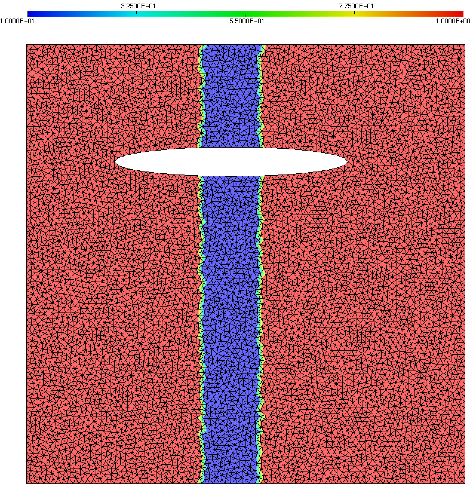
Prescribed size map

As the sol file has the same name than the mesh file, mmg reads it automatically by running the following command:

mmg2d_O3 hole.mesh

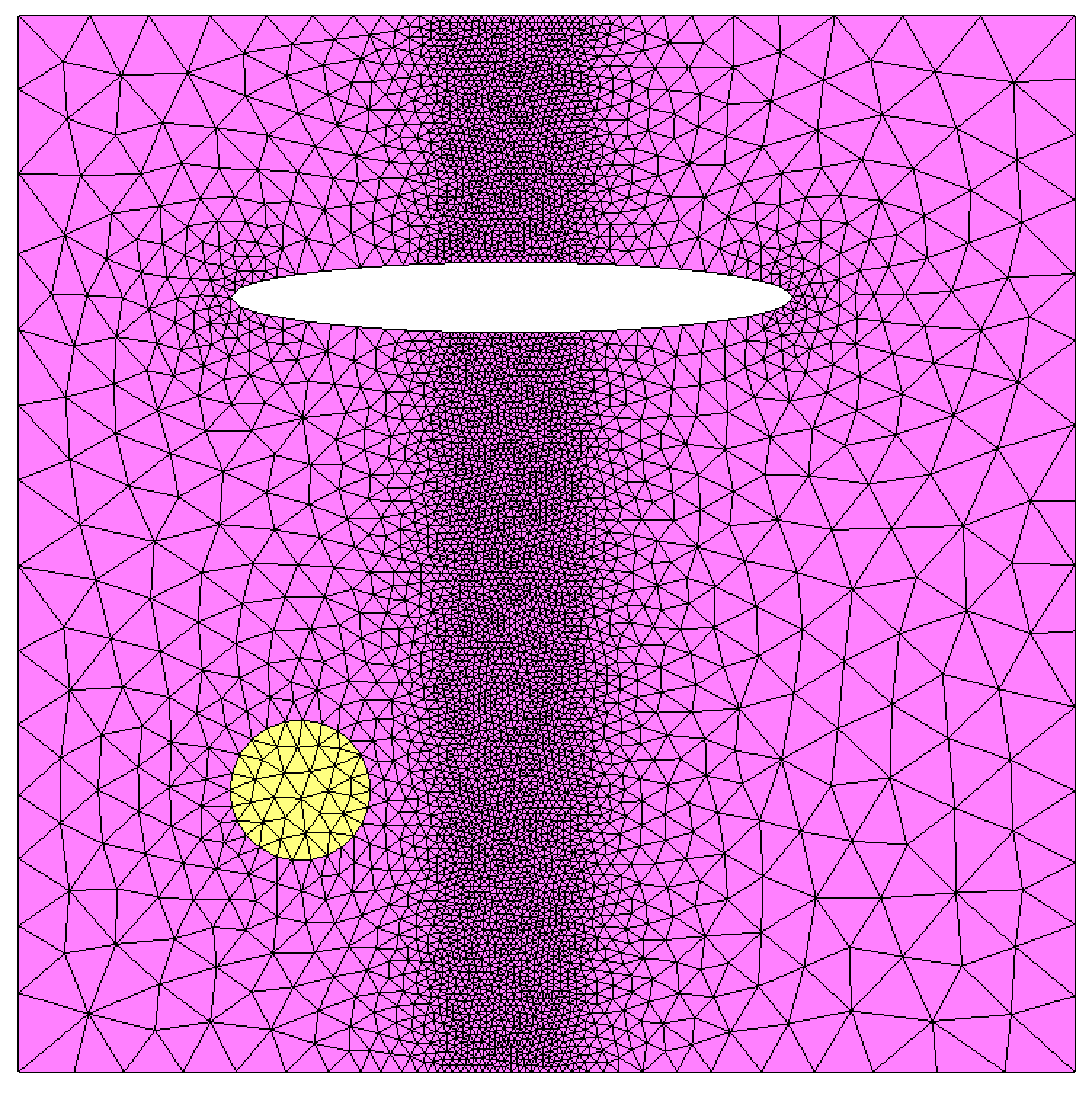
Adapted output mesh