Algorithm overview

Mesh adaptation algorithm

Goals

• Mesh modifications in agreement to a size map

• Generation of equilateral elements (possibly in a given metric)

Input data

A mesh and, eventually, nodal values prescribing the wanted edge sizes at each node (i.e. a size map).

Steps

1. Surface analysis

2. Rough surface mesh modifications for a good ‘samplig’ of the surface:

   • split too long edges (using patterns)

   • collapse too short edges

   • swap too bad elements

3. Size map construction:

   • intersection of the geometric (defined on boundaries) and user-prescribed (defined on the entire mesh) size maps

   • size map gradation with respect to the prescribed gradation parameter \(h_{\text{grad}}\): \(\frac{1}{h_{\text{grad}}} \leq \frac{l_1}{l_2} \leq h_{\text{grad}}\)

4. Fine surface mesh modifications with respect to the size map:

   • split (using patterns along the surface, and a Delaunay kernel inside the volume) or collape edges

   • swap edges belonging to too bad elements

   • vertex relocation to improve the quality

Isovalue discretization algorithm

Goals

Obtain an explicit mesh of a specific value of an implicit fonction

Input data

Nodal values of an implicit function (e.g. the signed distance function)

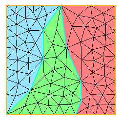
Figure 1: nodal values of a signed distance function at mesh nodes

Steps

1. Mark elements intersected by the level-set

2. For each marked element :

   • Mark the edges intersected by the level-set

   • Insert a new point at the intersection between the level-set and the edge(s)

   • Split the element using patterns and tag the boundary edge

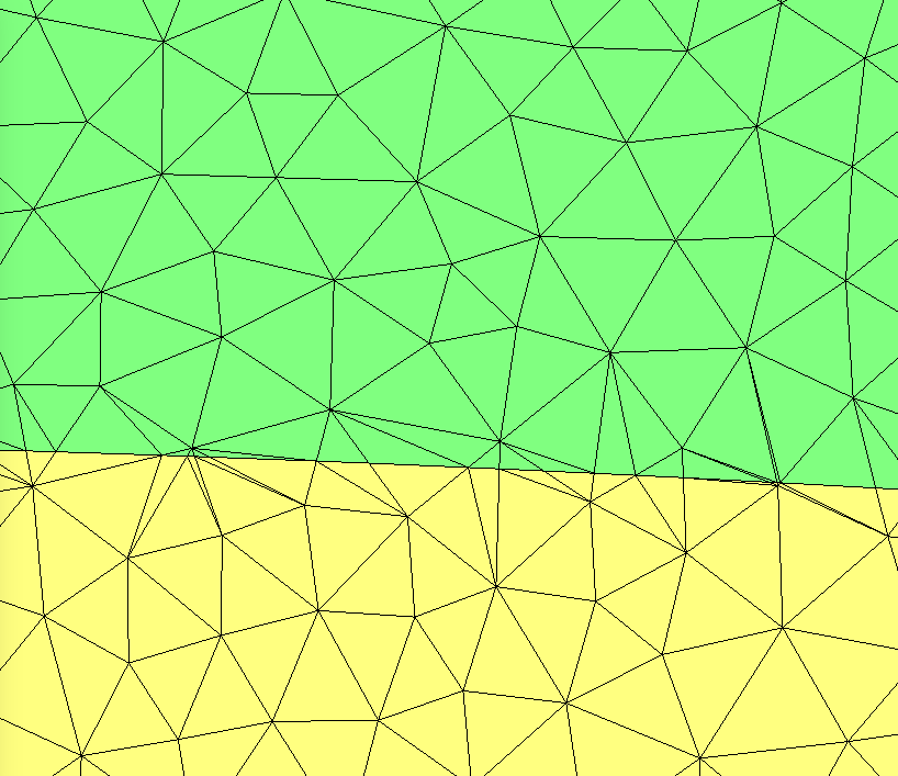
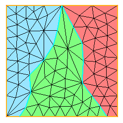
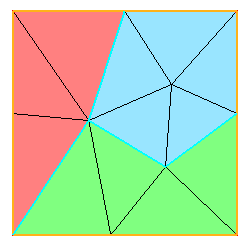
Figure 2: temporary mesh after the level-set discretization

3. Mesh improvement (using the mesh adaptation algorithm).

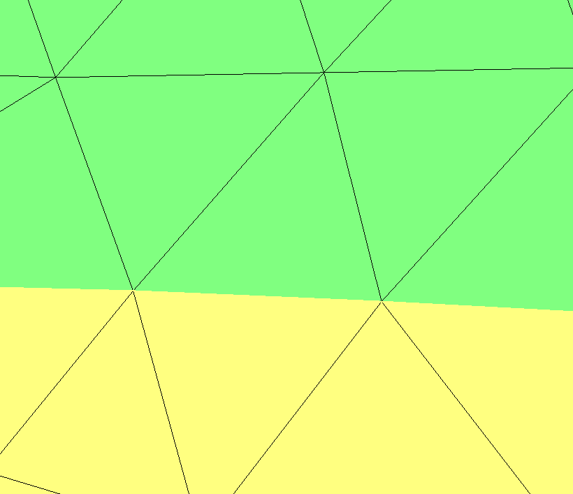
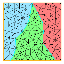
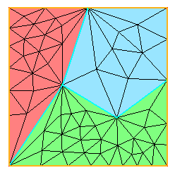
Figure 3: Output mesh

Lagrangian movement algorithm

Goals

Move an object inside a mesh keeping the mesh conformity.

Input data

Nodal values of the displacement (velocity) over boundaries of reference 10.

Steps

1. Extension of the velocity field:

   • Creation of a submesh containing 20 layers of elements around the boundary to move;

   • Propagation calling a linear elasticity solver with Dirichlet boundary conditions on the submesh;

2. Dichotomy loop:

   • Computation of the largest valid motion along the velocity field (with point relocation only);

   • Mesh motion;

   • Remeshing depending on the lagrangian mode (point relocation, point relocation + edge swapping, point relocation, edge swapping, point insertion and collapse);

3. go back to step 1.

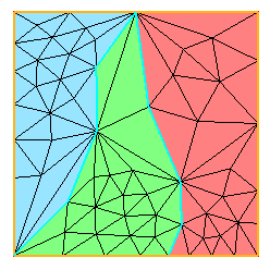
Distributed memory parallelization algorithm (ParMmg)

Goals

Mesh adaptation on distributed memory architectures

Steps

1. Mesh distribution: centralized input meshes are partitionned and distribued among available MPI ranks, distributed input meshes are rebalanced;

2. Mesh subdivision: on each processor, the mesh can be subdivided into sub-meshes (groups);

3. Mesh adaptation: the sequential remesher Mmg is called on each sub-mesh. Interfaces between the sub-meshes are not authorized to be modified (we say that those interfaces are constrained or frozen);

4. Interface migration: In order to be able to remesh the constrained interfaces, we create new sub-meshes using a front migration algorithm or a new call to a graph partitionner: interfaces that were frozen during the previous step should be inside the newly defined sub-meshes;

5. Go to step 3 until reaching the stop criterion (maximal number of iteration).